Configuring, Training, and Testing Models

A Model is built on a Predictor and includes the same target metric. Each Model has a subset of the agent and customer features present in the Dataset. The Feature Analysis report helps you to identify the features with the strongest impact on the target metric. You can create multiple Models for the same Predictor, each with a different set of features selected.

• You can compare how well Models work to create the most effective ones.
• You can configure Models that are best-suited to specific circumstances and control which Model is used by activating and deactivating them. This enables you to respond promptly to changes such as weekday vs weekend volume or the anticipated increase in certain types of interactions after a big marketing push.

When you create a Predictor, a full feature set Model is created automatically, including all the agent and customer features populated from the Predictor. A Predictor can have a number of Models associated with it.

• The right-hand toggle navigation menu enables you to view a tree view of all Datasets associated with your Account, with the Predictors and Models configured for each. To open or close this navigation menu, click the icon.
• You must reload the page to view updates made using the Predictive Routing API, such as appending data to a Dataset, creating, updating, or deleting a Predictor, or creating, updating, or deleting a Model.

Important

The full feature set Model comprises as complete a set of Local Models as possible based on the amount of data available for each agent (one Local Model per agent). If it's not possible to train a Local Model for a specific agent, GPR generates the following log message, indicating that the Local Model has been skipped for a specific agent, and omits that agent from the full feature set Model: WARNING <BOTTLE> models.py:420 RETRAIN: Skipping training for individual model <agent_id> since no data is available for classes.

For example, you might have a Boolean metric, such as FCR. If, for a specific agent, all entries from the training set had only examples of one Boolean class (that is, either all were resolved, or none were resolved), GPR cannot create a Local Model for that agent.

• You can configure a routing strategy to use a specific Predictor, then edit the Models and change which are active. In this way, routing can be adjusted and optimized on the fly, without requiring you to edit the strategy. For instructions on this specific functionality, see Activating multiple Models at once, below.
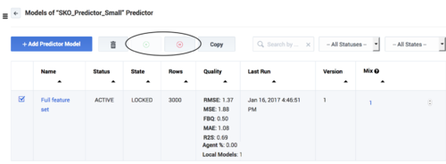
• The list of Models includes the Quality column, which provides analysis reports on Model Quality and Agent Coverage.

Creating and Configuring a New Model

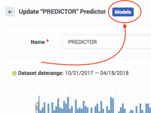
To open the configuration menu, click the Settings gear icon, located on the right side of the top menu bar: .

Procedure: Open the Models interface

Steps

To access your Models:

1. Select Predictor from the left-hand navigation bar and then click the name of a Predictor in your list.

   The Predictor configuration window opens.

2. Click Models.

Add a New Model

Procedure:

Steps

When you create a Predictor, GPR automatically adds the full feature set Model, as shown in this graphic. The full feature set Model is a Global model, created by default, that includes every Agent and Customer feature you selected when you created the Predictor.

• To create a new Model, click Add Predictor Model.

Configure a Model

Procedure:

Steps

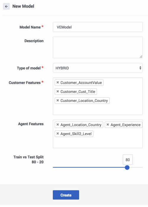
Edit the fields as explained below.

1. To choose Agent Features and Customer Features, click in the appropriate text box and select the desired features from the drop-down list.
   • Agent Features are items that refer to the agent. All agent-related fields in your selected Dataset appear in the Agent Features field.
   • Customer Features are items that refer to the customer or that are available in interaction user data. They refer to aspects of the environment, broadly speaking, in which the interaction occurs.

   Important

   You can only select from the Agent Features and Customer Features that are included in the Predictor.

2. To remove a feature, click the X in the box containing the feature name.
3. Choose one of the Model types, GLOBAL, DISJOINT, or HYBRID.

Global Model

• A single Model is built to predict agent scores.
• Provides generalizations that are probably true across the whole pool of agents. For example, agents that are part of this group might have a lower transfer rate; agents with longer tenure generally have higher resolution performance; and so on.
• Select this Model type only if there are action features that correlate with the target metric.
• In the absence of Agent Features, the Global Model type produces the same score for every agent, which makes it useless for ranking.

Disjoint Model

• A Model, also called a Local Model, is built for each agent.
• Captures agent-specific idiosyncrasies with respect to performance.
• With this option, a Global Model is also built to produce scores for agents for whom individual Models cannot be created. For example, some agents might not have enough data to create an individual Model.

Hybrid Model

• Combination of Global and Disjoint Models, which uses an average of their scores.
• Can both provide generalization and capture agent-specific nuances in performance.
• Select this Model only if there are Agent Features that correlate with the target metric; that is, the metric (first-contact resolution, net promoter score, average handle time, and so on) for which the associated Predictor is built.

Set the Training and Testing Percentages

Procedure:

Steps

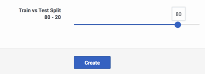
You can configure how much of your Dataset is used to train your Model and how much is used to test how well it works. This split is time-based. The most recent interactions are allocated to the test section of the Dataset. For example, if you use 80% of the data to train your Model and 20% to test it, the most recent 20% of the Dataset records are used for testing.

Important

Data used for training is not used to score agents. Agent scoring is based on the data in the Agent and Customer Profiles or, if you are using the GPR API, on data passed in the API score request as part of the context parameter. If both are present, data from the API request takes priority over data from the Agent and Customer Profiles.

To set this value:

1. Use your mouse to slide the indicator to the desired point on the Train/Test bar.

Train Your New Model or Retrain an Existing One

Procedure:

Steps

After you create your Model, you must train it on your data.

• When a trained Model has not been yet activated, you can modify it. For example, you might add new Agent or Customer Feature, change the train/test split, and so on. After those modifications, you must retrain your Model.
• When you train or retrain a Model, the integer in the Version column of the list of Models is incremented.
• If you change the date range for the Predictor data, then purge and regenerate your dataset, an already-trained Model does not need to be retrained. It uses the previously configured date range. But all Models created after the data purge and regeneration use the new date range.

1. Select the check box in the table row for your Model.
2. Click Train.

The Training job can take a fairly long time, depending on the size of your Dataset. Click the Jobs tab to monitor job progress.

Viewing Agent Coverage and Model Quality Reports

After you train your Model, the Quality column shows values for various methods of evaluating how well the Model works. The evaluation methods are selected automatically depending on the type of Model.

Procedure: View Model Quality and Agent Coverage reports

Steps

GPR provides the following analysis types:

• Classification analysis buckets observations into predetermined binary categories, based on data already used for training. In this case, you already know that the data can be divided into meaningful categories, into which your new data can be placed. For example, you might record interaction results showing whether a customer's issue was resolved or not; whether the desired AHT was met or not; whether the final NPS was above a certain value or not; and so on.
• Regression analysis attempts to determine the strength of the relationship between one dependent variable (usually denoted by Y) and a series of other changing variables (known as independent variables). For example, you might be evaluating how agents' language skill levels (independent, changing) affect their ability to achieve first contact resolution (the dependent variable).

How different Model types are evaluated for quality:

• For binary classification Models, which are evaluated using the area under the curve (AUC) method, you can analyze their effectiveness using a Receiver Operating Characteristic (ROC) Curve.
• Regression Models, such as those shown in the graphic, are evaluated by the following methods:
  • RMSE (Root-mean-square deviation)
  • MSE (Mean squared error)
  • FBQ (Fraction below quantile. Calculated as mean(y_i < y_pred_i), where y and y_pred are sequences of actual and predicted values, respectively.)
  • MAE (Mean absolute error)
  • R2s (R squared) indicates how closely the predictions fit with the historical observations. The values range from 1.0, the highest possible value, down. Use the following guidelines to interpret the level of success your predictions are achieving:
    • Score = 1.0: The best possible Model. This is an unlikely score in real-world situations.
    • Score between 0 and 1: The higher the score, the better your predictions. This is the range you can expect to encounter if your Models are correctly configured.
    • Score = 0.0: Indicates a blind Model; that is, a constant Model that always predicts the same expected value, disregarding the input features.
    • Score < 0: Off track. The score can be negative, without a fixed lower limit. If your results fall into this range, examine your Model for misconfiguration of some sort.
• Agent % - This agent coverage metric indicates how many Local Models were built for agents, as a function of the total agents available. It evaluates how much coverage a Model has. The agent coverage metric is available for Hybrid and Disjoint Model types.

  It is possible to have 0% coverage. This indicates that none of the agents included in the Agent Profile also have records in the Dataset that was used to train the Model. {A low Agent % value might indicate that you should upload more data.

  If the Predictor is configured with Dataset Generated and there is no Agent Profile configured, then the Agent % = -1.00. (Note that the Dataset Generated setting is not intended for use in production environments.)

  Whatever type of metric you are using--numeric or Boolean--GPR creates a Local Model for each agent for whom there is enough data. The description of Local Models immediately below explains what data is required to build a Local Model for an agent.

• Local Models - Displays the number of Local Models generated for agents in the Dataset on which the Predictor is built. Local Models are built only for Models that have the Hybrid or Disjoint type. For Global Models this metric is always 0. If a Model is new (that is, inactive and untrained) the metric value is -1.00 until the Model is trained. Once trained, the metric shows the actual number of Local Models.

  Keep in mind the following requirements:

  • For a numeric target metric, GPR creates a Local Model for each agent having at least one Dataset record (that is, who has handled at least one interaction that is included in the Dataset).
    • If the Predictor is configured with Dataset Generated and there is no Agent Profile configured, then the value for Local Models corresponds to the number of agents with interactions in the Dataset (for models of the Hybrid and Disjoint types) and Local Models = 0 (for Models of the Global type). (Note that the Dataset Generated setting is not intended for use in production environments.)
    • If you have configured an Agent Profile schema and there is an intersection between the agents who appear in the Agent Profile and the Dataset, the Agent % value is the number of agents in the Agent Profile who also have Local Models divided by the number of agents in the Agent Profile.

      For example, if there are a total of 10 agents in the Agent Profile but only one appears in the Dataset as well, the Agent % value = 10%, indicating that 10% of the agents in the Agent Profile have Local Models.

  • For a Boolean target metric, you must have at least one record per class (that is, one true/1 and one false/0) to build a Local Model. For example, take a Predictor using a Boolean target metric and based on a Dataset with 100 interactions and four agents. Agent1 handles one interaction only, so no Local Model is created. Agent2 handles two interactions but both has the value false for the target metric, so no Local Model is created. Agent3 and Agent4 handle two interactions each, with at least one metric value true and another false so Local Model are created for both.

ROC Model Quality Analysis

Procedure:

Steps

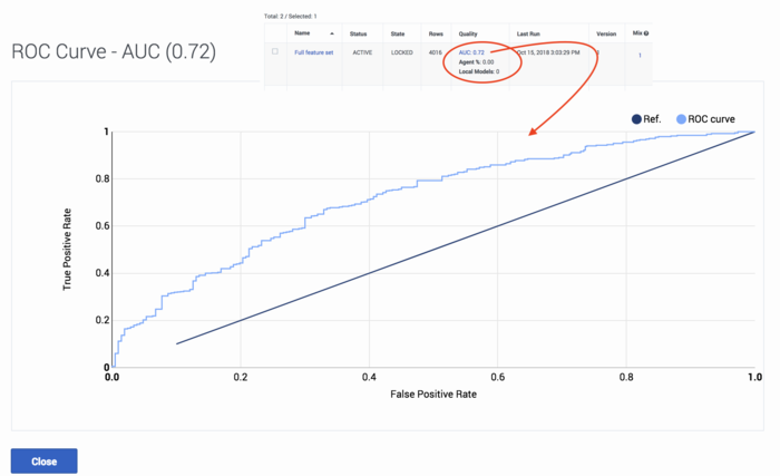
You can analyze the effectiveness of classification Models, which are evaluated by the area-under-curve (AUC) method, with a Receiver Operating Characteristic (ROC) Curve. This type of report is accessible only for classifier Predictors (Predictors that use a Boolean metric). Every trained Model for such a Predictor has an active AUC link in its row in the Predictors list.

• To open the Model Quality graph, click the AUC link in the Quality column.

  As you can see, the resulting diagram shows the ROC curve balancing the True Positive Rate and False Positive Rate. These terms, and some useful associated ones, are defined below:

  • True Positive (TP) - The number items that met the specified condition, and were predicted to meet the condition. In this case, a TP would be an interaction that met the designated CSAT level (value =true) and was predicted correctly to do so.
  • False Positive (FP) - The number of items that did not meet a condition, but were predicted to meet the condition. In this case, it would be interactions that were predicted to result in the specified CSAT level but did not.
  • False Negative (FN) - The number of items that did meet a condition, but were predicted not to meet the condition. In this case, it would be interactions that were predicted to result in an unsatisfactory CSAT level but did not.
  • Positive Population (PP) - The total number of interactions with a satisfactory CSAT (value = true).
  • Negative Population (NP) - The total number of interactions with an unsatisfactory CSAT (value = false).

  The diagram shows a curve outlining the items that were true positives—correct, positive predictions-—that occurred at a rate better than guesswork (the black line). The analysis looks at Model sensitivity versus specificity.

  • Sensitivity = TP/(TP + FN) = TP/PP - The ability of the test to detect the desired result.
  • Specificity = TN/(TN + FP) = TN / NP - The ability of the test to correctly rule out the condition where it doesn't occur.

The ROC curve is a way to see the tradeoff between sensitivity and (1 - specificity) for different thresholds of probability for classification. This is the preferred way to view Model Quality for classifiers.

Activating a Model

Procedure: Activate your Model

Steps

After your Model is trained, activate it to use it for routing.

1. Select the check box in the table row for your Model.
2. Click the Play button.
3. To deactivate a Model, click the Pause button.

Procedure: Activating multiple Models at once

Steps

You can test Model performance against other Models by activating multiple Models at once. You can then choose how much traffic is scored using each Model. Models are selected at random to score interactions, with the number scored by each Model dependent on how you weight the Model using the Mix parameter.

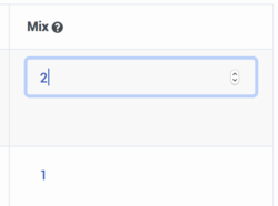
• In the Mix column, enter the desired numbers for each Model or set them using the up and down arrows located next to the number in the table cell.

  The numbers indicate the relative numbers of interactions that are scored using each Model. If you have a 1 in each column, the interactions are equally divided among the active Models. If you set 1 for Model A and 2 for Model B, Model B is used to route two interactions for every one using Model A.

  • For example, you might have three Models to which you have assigned the weights of 1, 8, and 4 in the Mix field. Think of these weights as creating three buckets of different sizes, with a total value equal to the three weight values added together:

    0 |_|______|___| 13

    On each incoming interaction, GPR chooses an entirely random number between 0 and the sum of all the weights (here this is 13). Depending on which bucket or range the chosen number falls in, the interaction is scored using the associated Model. In this example, Models are selected as follows:

    • If the number is between 0 - 1 (the first bucket), the interaction is scored using the first Model
    • If the number is between 2 - 9 (the second bucket), the interaction is scored using the second Model
    • If the number is between 10 - 13 (the third bucket), the interaction is scored using the third Model

    Given that the numbers are selected randomly, the number of interactions scored using each Model end up proportional over time to the weights you selected in the Mix field.

Editing Models

Procedure: Editing Models

Steps

You can only edit a Model that has not yet been activated.

• If a Model has been trained and edited after training, the Model needs to be retrained.

Once a Model has been activated, it can not be changed or edited again. Even if you stop (deactivate) it, the Model remains locked.

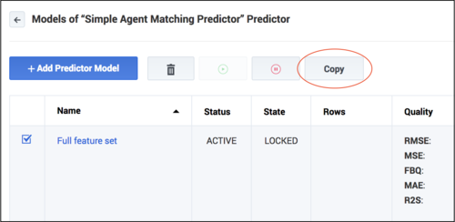
To edit an activated Model, copy it. Only an active, trained Model can be copied. When you make a copy, you are creating a new Model that has the same name as the original Model with the added suffix <copy><version number appended>.

1. Select the check box for the Model to be copied in the list of Models.

   The Copy button appears.

2. Click Copy.

   The copy appears in the list of Models.

3. Click the name of the copy and then follow the steps given above to edit, train, and activate the copy.